Forward Problem

Coupled Acoustic-Gravity wave equations:

Velocity: \(\boldsymbol{u}(\boldsymbol{x}, t)\), Pressure: \(p(\boldsymbol{x}, t)\),
Surface Height: \(\eta(\boldsymbol{x}, t)\)

Forward Problem

Coupled Acoustic-Gravity wave equations:

\[\begin{cases} \rho \frac{ \partial\boldsymbol{u}}{\partial t} + \nabla p = \boldsymbol{0}, \frac{1}{K} \frac{ \partial p}{\partial t} + \nabla \cdot \boldsymbol{u} = 0, & \Omega \times (0,T)\nonumber\\ p = \rho g \eta, \frac{ \partial\eta}{\partial t} = \boldsymbol{u} \cdot \hat{\boldsymbol{n}}, & \Gamma_s \times (0,T) \nonumber\\ \boldsymbol{u} \cdot \hat{\boldsymbol{n}} = -\frac{\partial b}{\partial t}, & \Gamma_b \times (0,T) \nonumber\\ \boldsymbol{u} \cdot \hat{\boldsymbol{n}} = Z^{-1} p, & \Gamma_a \times (0,T)\nonumber \end{cases} \]

bulk modulus \(K\), density \(\rho\), \(Z = \rho c\), \(c = \sqrt{K/\rho}\)
bathymetry \(b(\boldsymbol{x}, t)\); Homogeneous ICs

Bayesian Inverse Problem

Goal: determine posterior measure \(\mu_{\text{post}}\)

\(m\): model parameters - spatiotemporal field,
\(d\): obs. data - pointwise space, continuous time

Bayes Rule: \(\frac{\text{d}\mu_{\text{post}}}{\text{d}\mu_{\text{prior}}} \propto \pi_{\text{like}}(d|m) \)
\(=\exp\left(-\frac{1}{2}\|\mathcal{F}m - d\|_{\Gamma_{\text{noise}}^{-1}}^2\right)\) (in our case)

Parameter-to-Observable (p2o) Map:
\(\mathcal{F}: m \mapsto d\)

Linear Inverse Problem, Gaussian Prior

Prior: \(m \sim \mathcal{N}(m_{\text{prior}}, \Gamma_{\text{prior}})\)

Observations: \(d = \mathcal{F}m + \nu\), \(\nu \sim \mathcal{N}(0, \Gamma_{\text{noise}})\)

Posterior: \(\mu_{\text{post}} = \mathcal{N}(m_{\text{map}}, \Gamma_{\text{post}})\)

\[\begin{gather} \Gamma_{\text{post}}=\left(\mathcal{F}^* \Gamma_{\text{noise}}^{-1} \mathcal{F} + \Gamma_{\text{prior}}^{-1}\right)^{-1} \nonumber\\ m_{\text{map}}=\Gamma_{\text{post}}\left(\mathcal{F}^* \Gamma_{\text{noise}}^{-1} d + \Gamma_{\text{prior}}^{-1} m_{\text{prior}}\right) \nonumber \end{gather}\]

Linear Inverse Problem, Gaussian Prior

\[\begin{gather} \Gamma_{\text{post}}=\left(\mathcal{F}^* \Gamma_{\text{noise}}^{-1} \mathcal{F} + \Gamma_{\text{prior}}^{-1}\right)^{-1} \nonumber\\ m_{\text{map}}=\Gamma_{\text{post}}\left(\mathcal{F}^* \Gamma_{\text{noise}}^{-1} d + \Gamma_{\text{prior}}^{-1} m_{\text{prior}}\right) \nonumber \end{gather}\]

Want to find \(m_{\text{map}}\) and \(\Gamma_{\text{post}}\) in real-time

Stuart, Andrew M. "Inverse problems: a Bayesian perspective." Acta numerica 19 (2010): 451-559.

Finding the MAP Point

\(\Gamma_{\text{post}}^{-1} =: \mathcal{H} \) is the Hessian (of negative log-posterior)

Each Hessian action \(\mathcal{H}v\) requires 1 Forward PDE Solve and 1 Adjoint PDE Solve (traditionally)

Solving \( \mathcal{H}m_{\text{map}} = \mathcal{F}^* \Gamma_{\text{noise}}^{-1} d + \Gamma_{\text{prior}}^{-1} m_{\text{prior}} \) with CG requires \(\text{rank}(\mathcal{H})\) Hessian actions

Ghattas, Omar, and Karen Willcox. "Learning physics-based models from data: perspectives from inverse problems and model reduction." Acta Numerica 30 (2021): 445-554.

Finding the MAP Point

For hyperbolic systems, \(\mathcal{H}\) can have high rank \(\Rightarrow\) many PDE solves

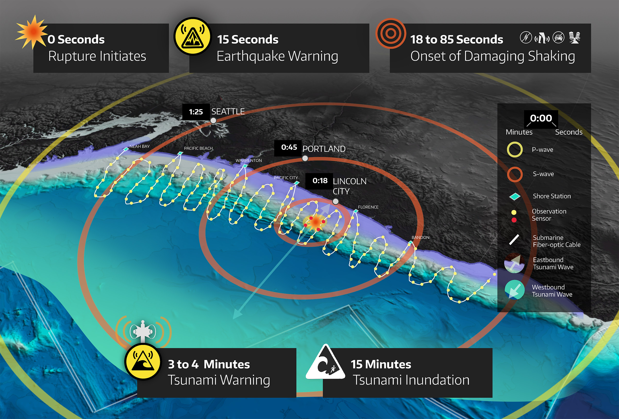
Cascadia Tsunami Problem:
\(\text{dim}(\mathbf{m}) \sim 10^{10}, \text{dim}(\mathbf{d}) \sim 10^6, N_t \sim 10^4\)
\(\Rightarrow\) \(\text{rank}(\mathbf{H}) \sim 10^4\)

\(\sim\) 1 hour / Hessian application \(\Rightarrow\) over 1 year (on thousands of nodes) for CG to converge!

Useless. We need to find the MAP point in seconds.

Real-Time Inference

Split computations into Offline and Online phases

Exploit (time) shift-invariance of autonomous dynamical systems

Real-Time Inference

Phase 1 (Offline): Construct p2o map from adjoint PDE solves

Phase 2 (Offline): Compute compact representation of \(\Gamma_{\text{post}}\)

Phase 3 (Online): Compute MAP point in real-time

Real-Time Inference

Phase 1 (Offline): Construct p2o map from adjoint PDE solves

Phase 2 (Offline): Compute compact representation of \(\Gamma_{\text{post}}\)

Phase 3 (Online): Compute MAP point in real-time

Real-Time Inference

Phase 1 (Offline): Construct p2o map from adjoint PDE solves

Recall: \( \mathbf{H} = \mathbf{F}^* \Gamma_{\text{noise}}^{-1} \mathbf{F} + \Gamma_{\text{prior}}^{-1}\)

shift-invariance \(\Rightarrow\) \(\mathbf{F}\) is block lower-triangular Toeplitz

Real-Time Inference

Phase 1 (Offline): Construct p2o map via adjoint solves

shift-invariance \(\Rightarrow\) \(\mathbf{F}\) is block lower-triangular Toeplitz

Real-Time Inference

Phase 1 (Offline): Construct p2o map via adjoint solves

shift-invariance \(\Rightarrow\) \(\mathbf{F}\) is block lower-triangular Toeplitz

Only one block row of \(\mathbf{F}^*\) needs to be computed/stored!

Real-Time Inference

Phase 1 (Offline): Construct p2o map from adjoint PDE solves

shift-invariance \(\Rightarrow\) \(\mathbf{F}\) is block lower-triangular Toeplitz

Real-Time Inference

Phase 1 (Offline): Construct p2o map from adjoint PDE solves

shift-invariance \(\Rightarrow\) \(\mathbf{F}\) is block lower-triangular Toeplitz

Real-Time Inference

Phase 1 (Offline): Construct p2o map from adjoint PDE solves

shift-invariance \(\Rightarrow\) \(\mathbf{F}\) is block lower-triangular Toeplitz

Real-Time Inference

Phase 1 (Offline): Construct p2o map from adjoint PDE solves

shift-invariance \(\Rightarrow\) \(\mathbf{F}\) is block lower-triangular Toeplitz

Real-Time Inference

Phase 1 (Offline): Construct p2o map from adjoint PDE solves

Adjoint PDE solved backwards in time with "source" at each observation point (\(\sim\)100 sensors)

Real-Time Inference

Phase 2 (Offline): Compute compact representation of \(\Gamma_{\text{post}}\) (through Sherman-Morrison-Woodbury)

Phase 3 (Online): Compute MAP point in real-time

Both rely on fast applications of \(\mathbf{F}\) and \(\mathbf{F}^*\)

Matvecs with Block Triangular Toeplitz Matrices

\(\mathbf{F} \) has \(N_t \times N_t\) blocks

Each block is \(N_d \times N_m\)

This is time-outer, space-inner indexing

Preprocessing: Reindex to space-outer, time-inner

Matvecs with Block Triangular Toeplitz Matrices

Preprocessing: Reindex to space-outer, time-inner

\(\mathbf{F} \) now has \(N_d \times N_m\) blocks

Each block is \(N_t \times N_t\)

Cascadia: \(N_d \sim 10^2, N_m \sim 10^{6}, N_t \sim 10^4\)

Matvecs with Block Triangular Toeplitz Matrices

Preprocessing: Reindex to space-outer, time-inner

\(\mathbf{F} \) now has \(N_d \times N_m\) blocks

Each block is \(N_t \times N_t\)

Each block of \(\mathbf{F} \) is now a lower-triangular Toeplitz matrix

Matvec Algorithm

Toeplitz matrix \(A\) is represented by its first column \(a_0\)

Embed \(A\) in a circulant matrix \(C\)

\(a_0\mapsto [a_0 \ \mathbf{0}]^T =: c_0\) (zero padding)

Input vector \(v \mapsto [v \ \mathbf{0}]^T =: u\)

\(C\) is diagonalized by the Fourier Transform

\(Cu = \text{IFFT}\left(\frac{1}{\sqrt{2n}} \text{FFT}(c_0) \odot \text{FFT}(u)\right)\)

\(Av\) is the first half of \(Cu\)

Matvec Algorithm

Toeplitz matrix \(A\) is represented by its first column \(a_0\)

Embed \(A\) in a circulant matrix \(C\)

\(a_0\mapsto [a_0 \ \mathbf{0}]^T =: c_0\) (zero padding)

Input vector \(v \mapsto [v \ \mathbf{0}]^T =: u\)

\(C\) is diagonalized by the Fourier Transform

\(Cu = \text{IFFT}\left(\frac{1}{\sqrt{2n}} \text{FFT}(c_0) \odot \text{FFT}(u)\right)\)

\(Av\) is the first half of \(Cu\)

Example

\(A = \begin{bmatrix} 1&0&0&0\\2&1&0&0\\3&2&1&0\\4&3&2&1\end{bmatrix}, v = \begin{bmatrix}5\\6\\7\\8\end{bmatrix}\)

\(a_0 = [1\ 2 \ 3 \ 4]^T \to [1\ 2\ 3\ 4\ 0\ 0\ 0\ 0]^T = c_0\)

\(u = [5\ 6\ 7\ 8\ 0\ 0\ 0\ 0]^T \)

Example

\(a_0 = [1\ 2 \ 3 \ 4]^T \to [1\ 2\ 3\ 4\ 0\ 0\ 0\ 0]^T = c_0\)

\(v = [5\ 6\ 7\ 8]^T \to [5\ 6\ 7\ 8\ 0\ 0\ 0\ 0]^T = u\)

\(\hat{c}_0 = [10,-1-9i,-2+2i, 3-3i, -2,\\ 3+3i, -2-2i, -1+9i]^T\)

\(\hat{u} = [ 26, 3+-21i, -2+2i, 7+-7i, -2,\\ 7+7i, -2+-2i, 3+21i]^T\)

Example

\(\hat{c}_0 = [10,-1-9i,-2+2i, 3-3i, -2,\\ 3+3i, -2-2i, -1+9i]^T\)

\(\hat{u} = [ 26, 3-21i, -2+2i, 7-7i, -2,\\ 7+7i, -2-2i, 3+21i]^T\)

\(\hat{c}_0 \odot \hat{u} = [260, -192-6i, -8i, -42i, 4,\\ 42i, 8i, -192+6i]^T\)

Example

\(\hat{c}_0 \odot \hat{u} = [260, -192-6i, -8i, -42i, 4,\\ 42i, 8i, -192+6i]^T\)

\[\begin{gather} \text{IFFT}\left(\frac{1}{\sqrt{8}} \hat{c}_0 \odot \hat{u}\right) = [5\ 16 \ 34 \ 60 \ 61 \ 52 \ 32 \ 0]^T \nonumber \\ \Rightarrow Av = [5\ 16 \ 34 \ 60]^T \nonumber \end{gather}\]

Example

FFT Method: \(Av = [5\ 16 \ 34 \ 60]^T \)

\[A = \begin{bmatrix} 1&0&0&0\\2&1&0&0\\3&2&1&0\\4&3&2&1\end{bmatrix}, v = \begin{bmatrix}5\\6\\7\\8\end{bmatrix}\]

\(\Rightarrow Av = [5\ 16 \ 34 \ 60]^T \checkmark\)

J. Demmel, P. Koev, and X. Li, “A Brief Survey of Direct Linear Solvers”. In Z. Bai, J. Demmel, J. Dongarra, A. Ruhe, and H. van der Vorst, editors. Templates for the Solution of Algebraic Eigenvalue Problems: A Practical Guide. SIAM, Philadelphia, 2000.

Matvec Algorithm

Recall: \(\mathbf{F} \) (reindexed) has \(N_d \times N_m\) Toeplitz blocks

Precompute (padded) FFTs of each block

Input vectors (reindexed): \(N_m\) blocks of \(N_t\) entries

FFTs (padded/batched) of input vectors

Elementwise multiply corresp. matrix/vector blocks

Sum results of each block row (local reduction)

IFFTs (batched) of results

Sum processor results (global reduction)

Matvec Algorithm

Precompute (padded) FFTs of each block

Input vectors (reindexed): \(N_m\) blocks of \(N_t\) entries

FFTs (padded/batched) of input vectors

Elementwise multiply corresp. matrix/vector blocks

Sum results of each block row (local reduction)

IFFTs (batched) of results

Sum processor results (global reduction)

Matvec Algorithm

FFT \(\to\) EWP \(\to\) L. Red. \(\to\) IFFT \(\to\) G. Red.

Same algorithm for \(\mathbf{F}^*\) — just complex conjugate the matrix FFT before the EWP

No extra storage or communication!

Roofline Analysis

85-95% memory bandwidth utilization on all kernels¹

¹Kernels below roofline are caused by small input size and correspond to < 1% of runtime. Profiled with NSight Compute.

Single-GPU Performance

Single-GPU Performance

Single-GPU Performance

Weak Scaling

Weak and Strong Scaling

Communication-Aware Partitioning

2D Partitioning: \(p = r\times c\) grid of GPUs

Goal: Minimize communication costs

Data-to-Parameter Ratio \(N_d/N_m\) is key

Cost Function:
\(C(r;p,N_d/N_m) = \)\(\frac{N_d}{N_m}\frac{1}{r}\log\frac{p}{r} + \frac{r}{p}\log r\)

Communication-Aware Partitioning

Cost Function:
\(C(r;p,N_d/N_m) = \)\(\frac{N_d}{N_m}\frac{1}{r}\log\frac{p}{r} + \frac{r}{p}\log r\)

Algorithm (\(k\) GPUs/node)

1. Compute \(\tilde{r} = \arg\min_r C(r;p,N_d/N_m)\)
2. If \(\tilde{r} = 1\text{ or } p,\) use \(r = \tilde{r}\)
3. Else, choose \(r\in \mathbb{Z}\) close to \(\tilde{r}\) so that \(r,\frac{p}{r} \in \mathbb{Z}\)
4. Try to ensure \(k|r\) and \(k|\frac{p}{r}\) (on-node vs. off-node)

Communication-Aware Partitioning

Real-Time Inference

Sherman-Morrison-Woodbury applied to \(\Gamma_{\text{post}}\):

\[ \begin{gather} \Gamma_{\text{post}}=\left(\mathcal{F}^* \Gamma_{\text{noise}}^{-1} \mathcal{F} + \Gamma_{\text{prior}}^{-1}\right)^{-1} \nonumber\\ =\Gamma_{\text{prior}}\left(I - \mathcal{F}^*\textcolor{BF5700}{\left(\Gamma_{\text{noise}} + \mathcal{F}\Gamma_{\text{prior}}\mathcal{F}^*\right)}^{-1}\mathcal{F}\Gamma_{\text{prior}}\right) \nonumber \end{gather} \]

\(\textcolor{BF5700}{\mathcal{K} = \Gamma_{\text{noise}} + \mathcal{F}\Gamma_{\text{prior}}\mathcal{F}^*}\)

Dense Matrix of size \(\sim 10^6\times 10^6\)

\(\Rightarrow\) Compress

Real-Time Inference

\[ \begin{gather} \mathbf{m}_{\text{MAP}}=\Gamma_{\text{prior}}\left(\mathbf{I} - \mathbf{F}^*\textcolor{BF5700}{\mathbf{K}}^{-1}\mathbf{F}\Gamma_{\text{prior}}\right)\mathbf{F}^*\Gamma_{\text{noise}}^{-1}\mathbf{d} \nonumber \end{gather} \]

Operations
\(\left(N_m \sim 10^6, N_d \sim 10^2, N_t \sim 10^4\right)\)

• \(2 \ \mathbf{F}^*\) matvecs — \(\mathcal{O}(N_dN_mN_t)\)
• \(1 \ \mathbf{F}\) matvec — \(\mathcal{O}(N_dN_mN_t)\)
• \(1 \ \textcolor{BF5700}{\mathbf{K}}\) solve — \(\mathcal{O}\left(N_d^2N_t^2\right)\) worst case
• \(2 \ \Gamma_{\text{prior}}\) solve — \(\mathcal{O}(N_mN_t)\)

Real-Time Inference

\[ \begin{gather} \mathbf{m}_{\text{MAP}}=\Gamma_{\text{prior}}\left(\mathbf{I} - \mathbf{F}^*\textcolor{BF5700}{\mathbf{K}}^{-1}\mathbf{F}\Gamma_{\text{prior}}\right)\mathbf{F}^*\Gamma_{\text{noise}}^{-1}\mathbf{d} \nonumber \end{gather} \]

Pointwise Variance \((\text{diag}(\Gamma_{\text{post}}))\) can be precomputed with stochastic estimators

Villa, Umberto, Noemi Petra, and Omar Ghattas. "HIPPYlib: an extensible software framework for large-scale inverse problems governed by PDEs: part I: deterministic inversion and linearized Bayesian inference." ACM Transactions on Mathematical Software (TOMS) 47.2 (2021): 1-34.